When a fit goes wrong

The boarding-school SIR model with a vague prior on the transmission rate: a prior predictive check that fails, chains that stick, why a noisy likelihood traps them, why more particles do not help, and the change of prior that fixes it, checked on simulated data.

Fitting the boarding-school outbreak fitted an SIR model to the 1978 boarding-school influenza counts and converged at the first attempt. It did so because the prior was placed on the basic reproduction number R_0. The more obvious choice is to put it on the parameter that appears in the infection rate, the transmission rate \beta, and to make it vague because we know little about \beta. This page makes that choice and follows the consequences: a prior that looks harmless implies epidemics nobody believes, two of four chains stop moving, and the diagnostics say so. We’ll work out why the chains stopped, see why the remedy the fit suggests does not cure it, and then check the fix on simulated data where we know the answer.

The data, model and sampler are those of the first page, and the commands run in a copy of the same directory, docs/guide/first-fit/.

A vague prior on the transmission rate

sir-beta.camdl differs from the first page’s model only in its parameters:

first-fit/sir-beta.camdl (excerpt)

parameters {
  #' transmission rate: infections per infected boy per day in a fully susceptible school
  beta  : rate ~ log_normal(mu = 0.0, sigma = 1.0)
  #' recovery rate; a boy stays infected 1 / gamma days on average
  gamma : rate ~ log_normal(mu = -0.69, sigma = 0.42)
  #' boys at risk
  N0    : count
  #' boys ill on day 0
  I0    : count
}

There is no let beta = R0 * gamma; \beta is estimated directly. Its prior is log-normal with median 1 per day and 90% of its weight between about 0.2 and 5.2 per day, a range wide enough that it seems to commit to nothing. The prior on \gamma, the recovery rate, is unchanged: a mean time infected of one to four days. The fit configuration, fit-beta.toml, is the first page’s with beta in place of R0.

The prior predictive check fails

Each prior looks reasonable on its own, but the epidemic depends on the two together, through R_0 = \beta/\gamma. Simulate 200 epidemics from the priors, as on the first page:

camdl simulate sir-beta.camdl --draws prior --fit fit-beta.toml -n 200 --seed 1 \
  --draws-out prior-beta.tsv -o prior-beta-runs.tsv
uv run plot_prior.py prior-beta.tsv prior-beta-runs.tsv data/in_bed.tsv prior-beta.svg

...
generated 200 prior draws from fit-beta.toml (2 estimated [0 fit-toml + 2 model-IR] + 2 fixed params)
...

Left: R0 = beta / gamma across 200 draws from the priors. Right: the number infected in each of the 200 simulated epidemics (blue), and the observed counts (black).

More than a quarter of the draws have R_0 below 1 (the left panel). An epidemic with R_0 below 1 dies out, because each case causes fewer than one more, and those draws are the flat lines along the bottom of the right panel. At the other end, draws with R_0 above 10 sweep through the school in two or three days. The fraction follows from the priors: \log R_0 = \log\beta - \log\gamma is normal with mean 0 + 0.69 and standard deviation \sqrt{1^2 + 0.42^2} \approx 1.08, so P(R_0 < 1) = \Phi(-0.69/1.08) \approx 0.26. A prior meant to describe an influenza outbreak in a school spends a quarter of its weight on outbreaks that never happen.

That would matter even if the sampler coped, because the posterior is a compromise between prior and data. It also matters for the sampler, because each chain starts from a draw from the prior.

The fit fails, and says so

camdl fit run fit-beta.toml --label beta --seed 4

...
  log L̂ mean = -74.8, sd σ = 1.95 (1000 particles, 20 pairs)
...
  acceptance ceiling 2·Φ(-s/2) = 0.3%   target 0.234 + 0.206/d = 33.7% (d = 2)
...
    Raise particles (σ ∝ 1/√N) if acceptance stays low, which is one remedy;
...
chain 0 1/3000  ll=-1362.5  acc=0%
chain 3 1/3000  ll=-558.6  acc=0%
chain 1 1/3000  ll=-319.5  acc=0%
chain 2 1/3000  ll=-124.7  acc=0%
...
chain 0 3000/3000  ll=-758.2  acc=0%
...
chain 1 3000/3000  ll=-228.5  acc=0%
...
chain 2 3000/3000  ll=-60.2  acc=38%
chain 3 3000/3000  ll=-59.9  acc=38%
...
  ✗ NOT converged — the chains are in different places
    max R̂ 3.325 (gamma), threshold 1.05
...
  chain  acceptance             λ end of warm-up  steps at floor
  0          0.050% ✗ too low           4.540e-5      241 / 1000
  1           0.10% ✗ too low           4.540e-5      365 / 1000
  2           39.6% ✓                   7.175e-1        0 / 1000
  3           40.2% ✓                   3.763e-1        0 / 1000
...
  ! chain 0: mean log_likelihood differs from the other chains' by -699.42 nats (Z = 1073.5 > 3.59), beyond what its standard error explains.
...

The fit runs to the end and then reports that it has not converged. Chains 0 and 1 accepted 0.05% and 0.1% of their proposals, a handful of moves in 3000 steps, while chains 2 and 3 accepted about 40%. \hat R is 2.25 for \beta and 3.3 for \gamma, far above camdl’s threshold of 1.05. The progress lines give each chain’s log-likelihood at its first and last step: chains 0 and 1 started at −1362 and −320, at parameter values whose epidemics look nothing like the data, and ended at −758 and −228, while chains 2 and 3 ended near −60. The traces in camdl ’scope show the same thing:

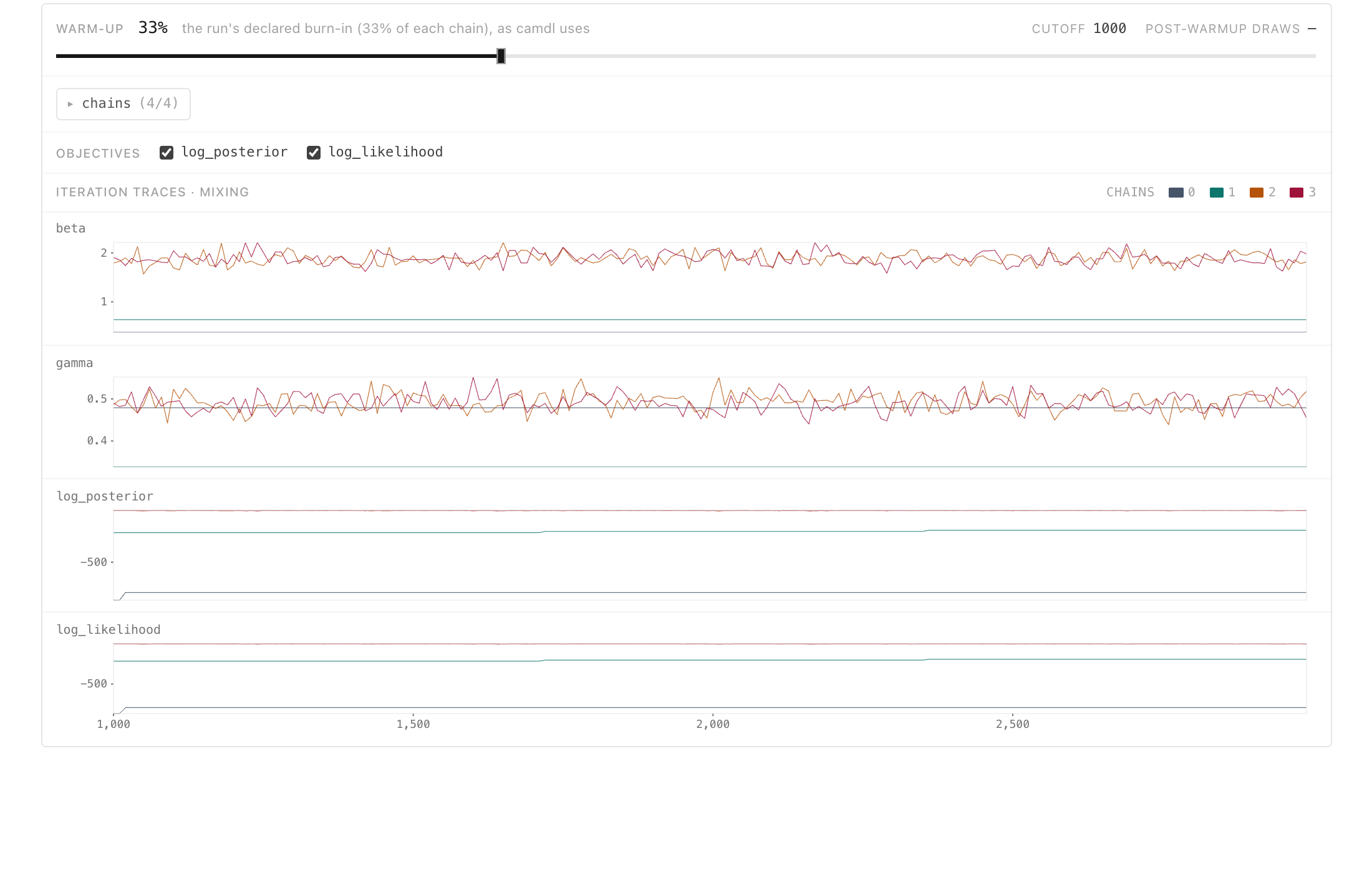
The `beta` fit in camdl ’scope, Traces tab, after burn-in. Chains 2 and 3 (orange and red) move over the same band, with \beta near 1.9 and \gamma near 0.49. Chain 1 (green) sits flat at \beta \approx 0.64, \gamma \approx 0.33, and chain 0 (grey) flat at the bottom of the \beta panel, each for the whole run; their log-likelihoods (bottom panels) stay far below those of chains 2 and 3.

The flat chains are not exploring a second answer. They did not move, and their log-likelihoods are hundreds of units below the moving chains’; even if there were a second mode where they sit, a gap that size would leave it a negligible share of the posterior. Both sit at a transmission rate well below the value of about 1.9 per day on which the moving chains agree.

Warning: Do not report an unconverged fit, or rerun it until it passes

When chains disagree like this, the pooled draws are a mixture of the posterior and wherever the stuck chains happen to be, and no summary of them is an estimate of anything. Rerunning with other seeds until one passes is not a remedy either: a fit that converges only for lucky seeds has not converged.

Why the chains stuck

PMMH, the sampler, is Metropolis–Hastings with the exact likelihood replaced by the particle filter’s estimate \widehat p(y\mid\theta). From the current value \theta it proposes \theta' from a proposal distribution q and accepts it with probability

\alpha = \min\!\left\{1,\; \frac{\widehat p(y\mid\theta')\,p(\theta')\,q(\theta\mid\theta')} {\widehat p(y\mid\theta)\,p(\theta)\,q(\theta'\mid\theta)}\right\},

where p(\theta) is the prior. The estimate at the proposal is fresh; the estimate at the current value is the one computed when the chain arrived there, and it is kept, not recomputed. That is what makes PMMH target the right posterior, and it is also its weak point. If the estimate at the current value happened to come out much too high, every later proposal is compared against that lucky number, and almost none can beat it.

How likely such a lucky number is depends on how noisy the estimate is, and that depends on where the chain is. camdl pfilter runs the particle filter at fixed parameters, and with --replicates it runs it repeatedly and reports the mean and standard deviation of the log-likelihood estimates. First, near where chains 2 and 3 mix:

camdl pfilter sir-beta.camdl --fit fit-beta.toml --particles 4000 --replicates 20 \
  --param beta=1.87 --param gamma=0.49 --param N0=763 --param I0=3

...
loglik = -58.6 ± 0.1 (20 replicates, N=4000)
...

Then at the point where chain 1 sits, read off the traces:

camdl pfilter sir-beta.camdl --fit fit-beta.toml --particles 4000 --replicates 20 \
  --param beta=0.64 --param gamma=0.33 --param N0=763 --param I0=3

...
loglik = -291.9 ± 19.1 (20 replicates, N=4000)
...

Both use four times the fit’s 1000 particles. Near the posterior, twenty estimates agree to within a fraction of a log unit. At chain 1’s point, where almost every simulated epidemic is improbable under the counts and a few carry all the weight, they scatter by about 19 units around −292. With the fit’s own 1000 particles, the filter at that point cannot even finish twenty runs: one of them puts all its weight on a single simulated epidemic (EssCollapsed), where the estimate is undefined, and pfilter stops.

camdl pfilter sir-beta.camdl --fit fit-beta.toml --particles 1000 --replicates 20 \
  --param beta=0.64 --param gamma=0.33 --param N0=763 --param I0=3

...
pfilter replicate 14 error: PFDegenerate { kind: EssCollapsed { last_ess: [1.2617556145979603, 1.1357472849712626, 1.0072701707400828] }, obs_window: 5, elapsed_s: 0.02437665 }

Chain 1 holds an estimate of −228.5, made with 1000 particles. That is more than three of the 4000-particle standard deviations above their mean: a lucky outlier. Its proposals, which are close to where it is, get fresh estimates from a distribution at least this wide, and almost none come out higher.

The rest follows. A chain whose proposals are all rejected looks to the sampler like a chain whose steps are too big, so during burn-in it shrinks the proposal scale toward its target acceptance rate. Smaller steps change nothing, and the scale falls to its floor (\lambda = 4.5\times10^{-5} in the acceptance table) and stays there. Chain 0 sits further out still, at −758.

Under the hood: How noisy can the likelihood estimate be before PMMH stops mixing?

Suppose the log of the likelihood estimate is normal with standard deviation \sigma, the same at every \theta. For proposals so small that the true likelihood barely changes, a move is accepted only when the fresh noise beats the noise held at the current value, and the acceptance rate tends to 2\Phi(-\sigma/\sqrt2) (Sherlock et al. 2015, “On the efficiency of pseudo-marginal random walk Metropolis algorithms”, Annals of Statistics 43(1):238–275). At \sigma = 1 that is 48%; at \sigma = 19 it is about 4\times10^{-41}. Doucet et al. (2015, “Efficient implementation of Markov chain Monte Carlo when using an unbiased likelihood estimator”, Biometrika 102(2):295–313) recommend choosing the particle count so that \sigma is between about 1 and 1.7 near the posterior.

Two departures from that idealization matter here. The noise is not the same everywhere: it is small near the posterior and enormous far from it, so a particle count tuned near the posterior says nothing about a chain that starts far away. And while the estimate of the likelihood is unbiased, its logarithm is biased low, by more the noisier it is, so the occasional high estimate that traps a chain is an outlier above even the mean of the log estimates. Inference in camdl describes the filter’s estimate and its effective sample size.

The noise check, and why more particles do not cure this

Before sampling, the fit ran the particle filter twenty times at the start values and at a nearby proposal; the first lines of the excerpt above are its report. It found a standard deviation of about 2 log units at the start values (\beta = 1.5, \gamma = 0.4), and a spread s of the difference between two estimates large enough that its ceiling on the acceptance rate, 2\Phi(-s/2), is far below the 33.7% target. Its advice was to raise the particle count.

That advice is about the point the check measured, not the points where chains 0 and 1 stuck. More particles do reduce the noise everywhere, roughly as one over the square root of their number, but the pfilter runs above show what four times as many leave at chain 1’s point: a standard deviation of 19 log units, where PMMH needs about 1. The same fit with 4000 particles:

camdl fit run fit-beta-4000.toml --label beta-4000 --seed 4

...
  log L̂ mean = -73.6, sd σ = 1.05 (4000 particles, 20 pairs)
...
  ✗ NOT converged — the chains are in different places
    max R̂ 1.589 (beta), threshold 1.05
...
  chain  acceptance             λ end of warm-up  steps at floor
  0           36.1% ✓                   9.152e-1        0 / 1000
  1           0.30% ✗ too low           4.540e-5       56 / 1000
  2           37.5% ✓                   7.598e-1        0 / 1000
  3           35.2% ✓                   4.357e-1        0 / 1000
...

At the start values the noise check now finds a standard deviation of about 1, half the 1000-particle figure, as one over the square root predicts. Yet one chain still sticks, accepting 0.3% of its proposals, and \hat R is still far above 1.05; the fit costs four times as much. The chains that mixed in the first fit did so with 1000 particles, so the particle count was never the limit near the posterior. The starts are the problem, and the starts come from the prior.

Put the prior on R_0

\beta is hard to have beliefs about: it is a rate of effective contacts per day. R_0 is the number epidemiologists reason with. So estimate R_0 and \gamma, and derive \beta from them, as the first page did:

first-fit/sir-r0.camdl (excerpt)

parameters {
  #' basic reproduction number: boys one case infects in a fully susceptible school
  R0    : positive ~ log_normal(mu = 1.0, sigma = 0.5)
  #' recovery rate; a boy stays infected 1 / gamma days on average
  gamma : rate ~ log_normal(mu = -0.69, sigma = 0.42)
  #' boys at risk
  N0    : count
  #' boys ill on day 0
  I0    : count
}

let N = S + I + R
let beta = R0 * gamma

R_0 gets a log-normal prior with median 2.7 and 90% of its weight between 1.2 and 6.2, and let beta = R0 * gamma computes the transmission rate. The transitions, observations and data are unchanged. Run the same check:

camdl simulate sir-r0.camdl --draws prior --fit fit-r0.toml -n 200 --seed 1 \
  --draws-out prior-r0.tsv -o prior-r0-runs.tsv
uv run plot_prior.py prior-r0.tsv prior-r0-runs.tsv data/in_bed.tsv prior-r0.svg

...
generated 200 prior draws from fit-r0.toml (2 estimated [0 fit-toml + 2 model-IR] + 2 fixed params)
...

The same prior predictive check with the prior on R0.

Now 2% of draws have R_0 below 1, and the simulated epidemics range from slow to fast without spending their weight on outbreaks that never start. The prior on R_0 uses one piece of knowledge the prior on \beta ignored, that this was an outbreak; Fitting the boarding-school outbreak discusses whether that is fair.

Modeling choice: Did the reparameterization fix the sampler, or the prior?

The prior. Writing \beta = R_0\gamma changes nothing about which epidemics the model can produce or how probable the counts are under each; the likelihood is the same function, expressed in other coordinates. What changed is the prior: the new one, transformed to (\beta, \gamma), puts far less weight on small \beta than the old one did. Because the chains start from prior draws, far fewer of them start where the filter is hopelessly noisy, and the posterior moves too, if only slightly, because the prior is part of it.

Two consequences follow. A prior written directly on \beta that implied the same distribution would have worked equally well; the reparameterization is a convenient way to state a prior you can defend, not a numerical trick. And a prior on R_0 makes stuck chains rarer, not impossible: a draw with R_0 near 1 and a long infectious period still gives a slow epidemic far from the data. When that happens, \hat R says so. Starting the chains from an earlier estimate rather than from the prior is the other remedy; Inference in camdl describes the options.

Check the fit on data where the answer is known

Before trusting the new configuration on the real counts, check that it recovers parameters we chose. truth.toml sets R_0 = 3.75 and \gamma = 0.4, a mean of 2.5 days infected, with the school’s population and three initial cases. Simulate one epidemic from it, and fit that epidemic with fit-synthetic.toml, which is fit-r0.toml with its data file changed to synthetic.tsv:

camdl simulate sir-r0.camdl --params truth.toml --seed 7 --obs-only synthetic.tsv
camdl fit run fit-synthetic.toml --label synthetic --seed 1

...
observations written to synthetic.tsv
...
  chain 2: start 1 of 10 refused by the filter (EssCollapsed { last_ess: [1.0008017575775947, 1.0123020044324018, 1.0935745745950045] } at obs_window=5 after 0.03s); drawing another
  chain 2: start 2 of 10 refused by the filter (EssCollapsed { last_ess: [1.7106460440322144, 1.5096391498731223, 1.0244331399505382] } at obs_window=9 after 0.05s); drawing another
...
  ✓ converged
    max R̂ 1.004 (gamma), threshold 1.05
...
  R̂: below 1.05 counts as converged; above 1.1 draws a finding, a warning up to 1.5
...
  0           33.4% ✓                    1.021e0        0 / 1000
  1           28.1% ✓                    1.199e0        0 / 1000
  2           33.1% ✓                    1.108e0        0 / 1000
  3           35.8% ✓                   9.027e-1        0 / 1000
...
  R0           Rhat=1.002 ✓ ESS bulk=700 tail=773 (87.6% of 800 draws)
  gamma        Rhat=1.004 ✓ ESS bulk=776 tail=694 (97.0% of 800 draws)
...

Two of chain 2’s prior draws were rejected before sampling began (the refused lines). At those parameters the simulated epidemics were so far from the data that the particle filter’s weight collapsed onto one or two particles (EssCollapsed), the condition under which the estimate is useless. camdl refuses such a start and draws another, which keeps the worst starts out of the chains without hiding that it happened. All four chains then accept about a third of their proposals, and \hat R is at most 1.004.

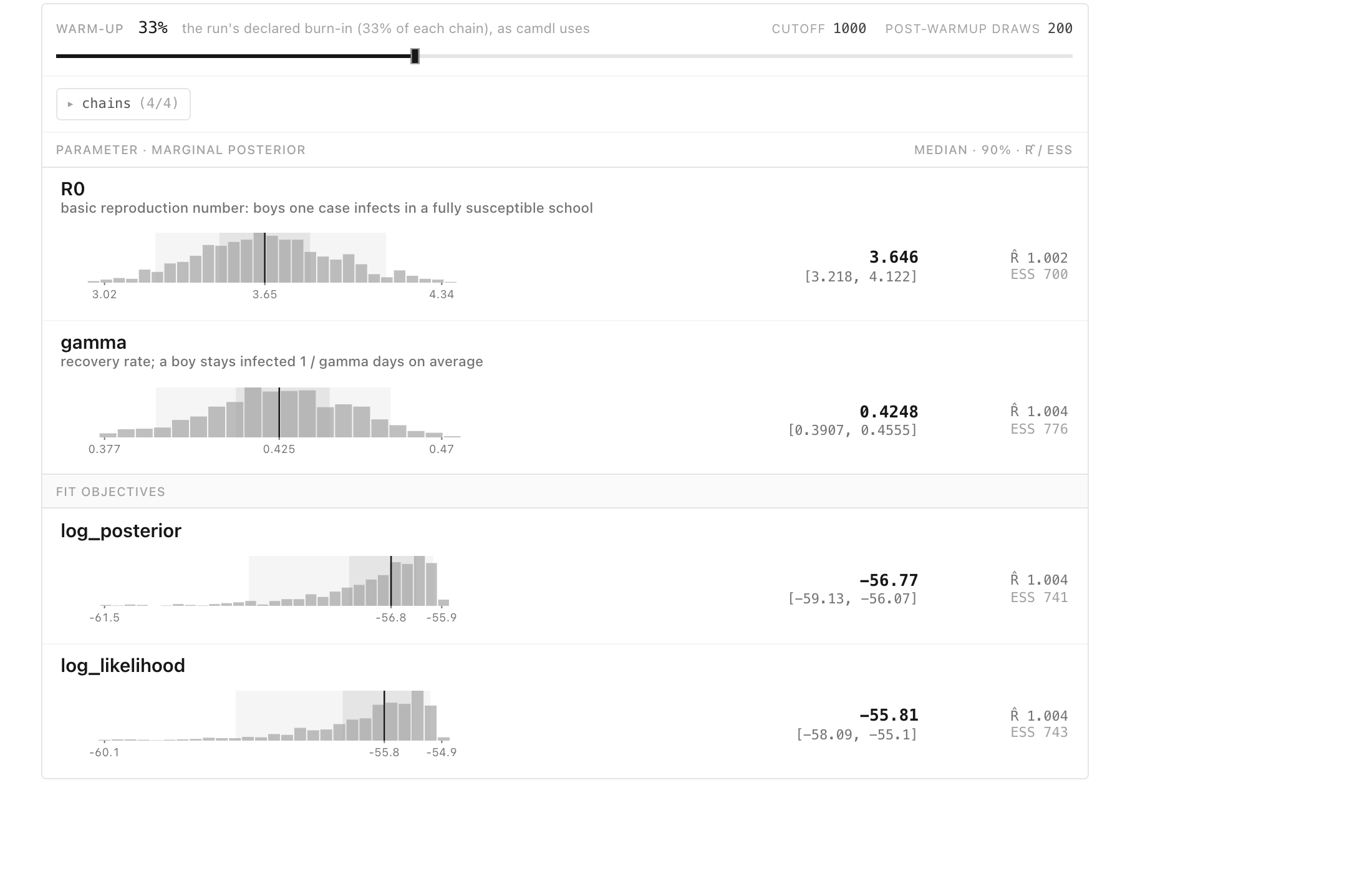
The synthetic fit in camdl ’scope, Posterior tab: the marginal posterior of each parameter, with its median, 90% interval, \hat R and ESS.

The true values lie inside both 90% intervals: R_0 = 3.75 against an interval of 3.22 to 4.12, and \gamma = 0.4 against 0.391 to 0.456. The fit recovers what it should. This shows that the sampler, the particle filter and the configuration work when the model is right; it says nothing about whether the model is right for the real school, because the simulated data came from the model itself. One recovery from one simulated epidemic is also a single check, not a demonstration that the 90% intervals cover the truth 90% of the time. The reasoning behind the fit workflow says more.

The same seed, now converged

Finally, the real counts, with the seed whose beta fit failed:

camdl fit run fit-r0.toml --label r0 --seed 4

...
  acceptance ceiling 2·Φ(-s/2) = <0.1%   target 0.234 + 0.206/d = 33.7% (d = 2)
...
chain 0 1/3000  ll=-190.1  acc=0%
chain 3 1/3000  ll=-698.2  acc=0%
chain 1 1/3000  ll=-240.1  acc=0%
chain 2 1/3000  ll=-113.0  acc=0%
...
  ✓ converged
    max R̂ 1.002 (R0), threshold 1.05
...
  R̂: below 1.05 counts as converged; above 1.1 draws a finding, a warning up to 1.5
...
  chain  acceptance             λ end of warm-up  steps at floor
  0           35.9% ✓                   7.229e-1        0 / 1000
  1           34.2% ✓                   5.043e-1        0 / 1000
  2           37.5% ✓                   8.283e-1        0 / 1000
  3           35.1% ✓                   4.342e-1        0 / 1000
...
  R0           Rhat=1.002 ✓ ESS bulk=473 tail=589 (59.2% of 800 draws)
  gamma        Rhat=1.001 ✓ ESS bulk=471 tail=583 (58.8% of 800 draws)
...

All four chains now accept 34% to 38% of their proposals and every \hat R is within 0.01 of 1. They started from prior draws at log-likelihoods between about −700 and −110, and all of them found their way to the posterior.

The noise check still fires, with an even lower ceiling than before. The start values are the same point as before, so the noise there is the same; what differs is the proposal the check happened to draw. The chains did not stay at that point, and their acceptance rates, measured on the run itself, are what to believe. That is the general lesson of this page: the pre-run check is a diagnosis at one point, and the end-of-run diagnostics, acceptance per chain, \hat R, and the chains’ log-likelihoods side by side, are the verdict. Diagnosing a fit covers the failures this example did not reach, and Checking and comparing models turns from whether the fit worked to whether the model is right.