Fitting the boarding-school outbreak
In January 1978 influenza swept through a boarding school in the north of England. Of 763 boys, 512 fell ill within two weeks, and the school recorded how many were confined to bed each day. We’ll fit a stochastic SIR model to those fourteen counts, estimate how fast the infection spread and how long a boy stayed ill, check that the sampler converged, and then ask whether the fitted model reproduces the data it was fitted to.
The fit is Bayesian: we state what we believe about the parameters before seeing the counts (the prior), and camdl combines that with the counts into a posterior. The page assumes you know what an SIR model is and have met Bayes’ rule; it does not assume you have used camdl before.
Every command on this page ran when the site was built, and the output under it is what camdl printed. The files are in docs/guide/first-fit/ in the camdl repository. To follow along, copy that directory, install camdl (Installing camdl), and run the commands from inside it.
The data: boys in bed each day
first-fit/data/in_bed.tsv
time	in_bed
0	3
1	8
2	26
3	76
4	225
5	298
6	258
7	233
8	189
9	128
10	68
11	29
12	14
13	4
time counts days from Sunday 22 January 1978, and in_bed is the number of boys confined to bed that day. The outbreak was reported in the British Medical Journal (Anonymous 1978, “Influenza in a boarding school”, BMJ 1(6112):587). The note gives 763 boys at risk, three boys in the college infirmary on 22 January, 512 boys ill in all, and influenza A (H1N1) isolated from six of the eight boys swabbed. The daily counts were read from the note’s graph and are distributed as the influenza_england_1978_school dataset of the R package outbreaks.
The model: an SIR epidemic and a Poisson count
first-fit/sir-r0.camdl
#' SIR model of the 1978 influenza outbreak at an English boarding school.
#'
#' Susceptible boys (S) are infected (I) by contact with infected boys and
#' recover (R). The school is a closed population of N0 = 763. The model is
#' fitted to one stream: the number of boys confined to bed each day.
#'
#' The prior is on R0 = beta / gamma instead of beta; Poisson counts around
#' the number infected.

time_unit = 'days

compartments { S, I, R }

parameters {
  #' basic reproduction number: boys one case infects in a fully susceptible school
  R0    : positive ~ log_normal(mu = 1.0, sigma = 0.5)
  #' recovery rate; a boy stays infected 1 / gamma days on average
  gamma : rate ~ log_normal(mu = -0.69, sigma = 0.42)
  #' boys at risk
  N0    : count
  #' boys ill on day 0
  I0    : count
}

let N = S + I + R
let beta = R0 * gamma

transitions {
  infection : S --> I  @ beta * S * I / N
  recovery  : I --> R  @ gamma * I
}

init {
  S = N0 - I0
  I = I0
}

observations {
  in_bed {
    columns       { time : time, in_bed : count }
    projected     = I
    emit_schedule = every 1 'days
    in_bed        ~ poisson(rate = projected)
  }
}

quantities {
  days_ill    = final(1 / gamma)           # mean time infected
  attack_rate = final((N0 - S) / N0)       # fraction of the school infected
  peak_in_bed = max(I)
  peak_day    = time_of_max(I)
}

simulate {
  from = 0 'days
  to   = 13 'days
  dt   = 0.1 'days
}
The school is a closed population: every boy is susceptible (S), infected (I) or recovered (R), and nobody arrives or leaves during the two weeks. Infection happens at total rate \beta S I / N and recovery at rate \gamma I, so a boy stays infected for 1/\gamma days on average. Rather than estimate the transmission rate \beta directly, the model estimates the basic reproduction number R_0, the number of boys one case would infect in a fully susceptible school, and computes \beta = R_0\gamma with a let. The two descriptions give the same epidemics; R_0 is simply the parameter people have beliefs about. When a fit goes wrong shows what happens with the prior on \beta instead.
The model is stochastic. camdl’s chain_binomial backend, which the fit configuration below selects, moves whole boys between compartments in small time steps (dt = 0.1 days), drawing how many are infected and how many recover in each step, so two runs with the same parameters give different epidemics. This matters for a school of 763: early on, with three boys infected, chance decides whether the outbreak takes off quickly or slowly.
The ~ after each estimated parameter gives its prior. Both are log-normal, which keeps a parameter positive; mu and sigma are the mean and standard deviation of its logarithm. The prior on R_0 has median e^{1}\approx2.7 with 90% of its weight between 1.2 and 6.2. The prior on \gamma comes from the BMJ note: boys spent three to seven days away from class and went back two to four days after they were allowed up, so a boy was in bed for roughly one to four days. The prior puts the mean time infected, 1/\gamma, at a median of two days, with 90% of its weight between one and four.
What camdl computes from it
The observations block connects the model to the data. Write x for the unobserved epidemic history, the number of boys in each compartment at every time, y_t for the number in bed on day t, and \theta = (R_0, \gamma). The stream in_bed takes the number infected, I_t(x), as the expected count on day t, and scores the observed count with a Poisson distribution around it. The likelihood of the fourteen counts is
p(y_{0:13}\mid\theta) = \int p(x\mid\theta)\, \prod_{t=0}^{13} \operatorname{Poisson}\!\bigl(y_t \mid I_t(x)\bigr)\,dx .
The first factor, the process model, says which epidemics the SIR dynamics can produce at these parameters. The product, the observation model, says how probable the recorded counts are if one particular epidemic happened. The integral averages over every epidemic we did not observe. No formula evaluates it, so camdl estimates it by simulation, and the estimate is noisy; that noise is what goes wrong on the next page.
The posterior is then p(\theta\mid y) \propto p(y\mid\theta)\,p(\theta), with p(\theta) the prior. Two simplifications are built into this likelihood, and both deserve a sentence before we rely on it. Treating “in bed” as “infected” assumes every infected boy was in bed, and the Poisson distribution assumes the counts scatter around I_t no more than a Poisson count does. Checking and comparing models tests both.
The quantities block names numbers to report from each simulated epidemic without fitting them: the mean time infected, the fraction of the school ever infected, and the size and day of the peak. simulate sets the window, day 0 to day 13. A tour of the language describes each block. Check that the model compiles:
camdl check sir-r0.camdl
✓ no errors, 0 warningsThe prior predictive check: what epidemics do the priors imply?
A prior on parameters is also a claim about epidemics, and it is easier to judge the claim than the parameters. Simulate 200 epidemics, each from a different draw of the priors, and plot them against the data:
camdl simulate sir-r0.camdl --draws prior --fit fit-r0.toml -n 200 --seed 1 \
  --draws-out prior-r0.tsv -o prior-r0-runs.tsv
uv run plot_prior.py prior-r0.tsv prior-r0-runs.tsv data/in_bed.tsv prior-r0.svg
...
generated 200 prior draws from fit-r0.toml (2 estimated [0 fit-toml + 2 model-IR] + 2 fixed params)
...--draws prior draws the estimated parameters from their priors (--fit names the fit.toml, described below, that says which parameters those are), and each draw is simulated once. --draws-out writes each draw’s parameters and -o the simulated trajectories, which plot_prior.py, a short script run with uv, plots.
The simulated epidemics range from slow ones that are still rising on day 13 to fast ones that peak within a few days, and the observed epidemic sits inside that range. Only a few draws have R_0 below 1, the flat lines along the bottom of the right panel. Nothing in the prior was tuned to the observed curve. That is what a prior should look like: it rules out what we know to be impossible and leaves the data to decide among the rest.
The fit configuration
first-fit/fit-r0.toml
[model]
camdl = "sir-r0.camdl"

[data.observations]
in_bed = "data/in_bed.tsv"

[estimate]
R0    = { start = 3.75 }
gamma = { start = 0.4 }

[fixed]
N0 = 763
I0 = 3

[method]
algorithm  = "pmmh"
backend    = "chain_binomial"
chains     = 4
particles  = 1000
iterations = 3000
burn_in    = 1000
A fit.toml names the model, binds each observation stream to its data file, and says which parameters to estimate and which to hold fixed. R_0 and \gamma are estimated with the priors from the model; the population and the three boys ill on day 0 are fixed at the numbers the BMJ note reports. The fit.toml reference lists every key.
The [method] table chooses particle marginal Metropolis–Hastings, pmmh (Andrieu, Doucet and Holenstein 2010, “Particle Markov chain Monte Carlo methods”, Journal of the Royal Statistical Society B 72(3):269–342). It is a Markov chain Monte Carlo (MCMC) sampler: each chain is a random walk through parameter values that, step by step, proposes a value near the current one, estimates the likelihood there, and accepts or rejects the move by comparing prior times likelihood at the two values. Over many steps the values a chain visits pile up in proportion to the posterior. The likelihood is estimated by a particle filter that runs 1000 simulated epidemics (particles) alongside the data.
Each of the four chains starts from its own draw from the prior. The first 1000 steps of each (burn_in) still remember where the chain started, and camdl uses them to tune the size of its proposals and then discards them. If the four chains, started in different places, end up describing the same distribution, that is evidence the answer does not depend on where they began. The start values are not where the chains begin: they are the point where camdl measures the particle filter’s noise before sampling.
The fit
camdl fit run fit-r0.toml --label r0 --seed 4...
✓ converged
max R̂ 1.002 (R0), threshold 1.05
...
R̂: below 1.05 counts as converged; above 1.1 draws a finding, a warning up to 1.5
...
chain acceptance λ end of warm-up steps at floor
0 35.9% ✓ 7.229e-1 0 / 1000
1 34.2% ✓ 5.043e-1 0 / 1000
2 37.5% ✓ 8.283e-1 0 / 1000
3 35.1% ✓ 4.342e-1 0 / 1000
...
R0 Rhat=1.002 ✓ ESS bulk=473 tail=589 (59.2% of 800 draws)
gamma Rhat=1.001 ✓ ESS bulk=471 tail=583 (58.8% of 800 draws)
...The fit prints a long log; the excerpt above keeps its verdict. --label r0 names the run so later commands can refer to it as @r0, and --seed makes it reproducible. The full log also carries a warning from a check of the particle filter’s noise made before sampling starts; When a fit goes wrong explains it, and the acceptance rates above show that here it did not come true.
Three numbers say whether the chains did their job. The acceptance rate is the fraction of proposals each chain accepted. camdl aims for about a third and calls 15% to 50% healthy; a chain that accepts almost nothing is not moving. \hat R (“R-hat”) compares the spread of draws within each chain with the spread between chains, and is close to 1 when the chains agree. camdl reports the rank-normalized version of Vehtari et al. (2021, “Rank-normalization, folding, and localization: an improved \hat R for assessing convergence of MCMC”, Bayesian Analysis 16(2):667–718) and calls a fit converged below 1.05; Vehtari et al. recommend the stricter 1.01. The effective sample size (ESS) says how many independent draws the 800 kept draws (4 chains × 2000 steps after burn-in, keeping every tenth) are worth, since successive steps of a chain are correlated. Here every chain accepts about a third of its proposals, \hat R is within 0.01 of 1, and the bulk ESS of each parameter clears the 400 that Vehtari et al. ask for before trusting \hat R with four chains.
camdl fit summary reads a finished fit and reports the estimates:
camdl fit summary @r0compiling sir-r0.camdl...
compiling sir-r0.camdl...
compiling sir-r0.camdl...
results/fits/fit_r0-b7a62cb1/pmmh-8d6841d6/seed_4-12c4a153/
SIR model of the 1978 influenza outbreak at an English boarding school. Susceptible boys (S) are infected (I) by contact with infected boys and recover (R). The school is a closed population of N0 = 763. The model is fitted to one stream: the number of boys confined to bed each day. The prior is on R0 = beta / gamma instead of beta; Poisson counts around the number infected.
camdl 0.1.0+f7e5c44 · pmmh · 4 chains · 800 draws · loglik -58.6 at the highest log-posterior draw (natural-scale prior, no Jacobian)
seeded from: from_prior (one independent draw per chain)
✓ converged
max R̂ 1.002 (R0), threshold 1.05
0 of 2 parameters above threshold · chains' log-likelihoods agree
0/800 forkable
── posterior ───────────────────────────────────────────────────────────────
param mean ESS bulk ESS tail R̂
R0 3.807 473 589 1.002
gamma 0.4927 471 583 1.001
── convergence ─────────────────────────────────────────────────────────────
param bulk folded classic worse per-chain ESS
R0 1.001 1.002 0.998 folded 139 64 200 95
gamma 1.001 0.999 0.999 bulk 132 68 139 111
acceptance = 0.357 (mean across chains)
ESS/iter = 0.0588 (min-param ESS 471 / 8000 raw sampling iters)
ESS/sec = 2.04 (min-param ESS 471 / 230.4s wall)
── chains ──────────────────────────────────────────────────────────────────
chain mean loglik Δ others Z flag
0 -59.47 +0.04 0.39
1 -59.60 -0.13 1.30
2 -59.44 +0.07 0.84
3 -59.48 +0.02 0.24
--parameters for priors and provenance · --explain for how to read thisThe posterior mean of R_0 is about 3.8, and of \gamma about 0.49, a mean of a little over two days infected. The chains table compares each chain’s mean log-likelihood with the other chains’; Z divides the gap by its Monte Carlo standard error, and none is large enough to flag. A chain stuck somewhere else would sit tens or hundreds of log-likelihood units away.
These numbers summarize the chains; the chains themselves are worth a look. camdl ’scope is a viewer for fits that runs in your browser. Started with camdl-scope --port 8800 in the directory you are working in, it lists every fit under results/fits/ and refreshes them while they run. Its Traces tab plots each parameter at every step of every chain:
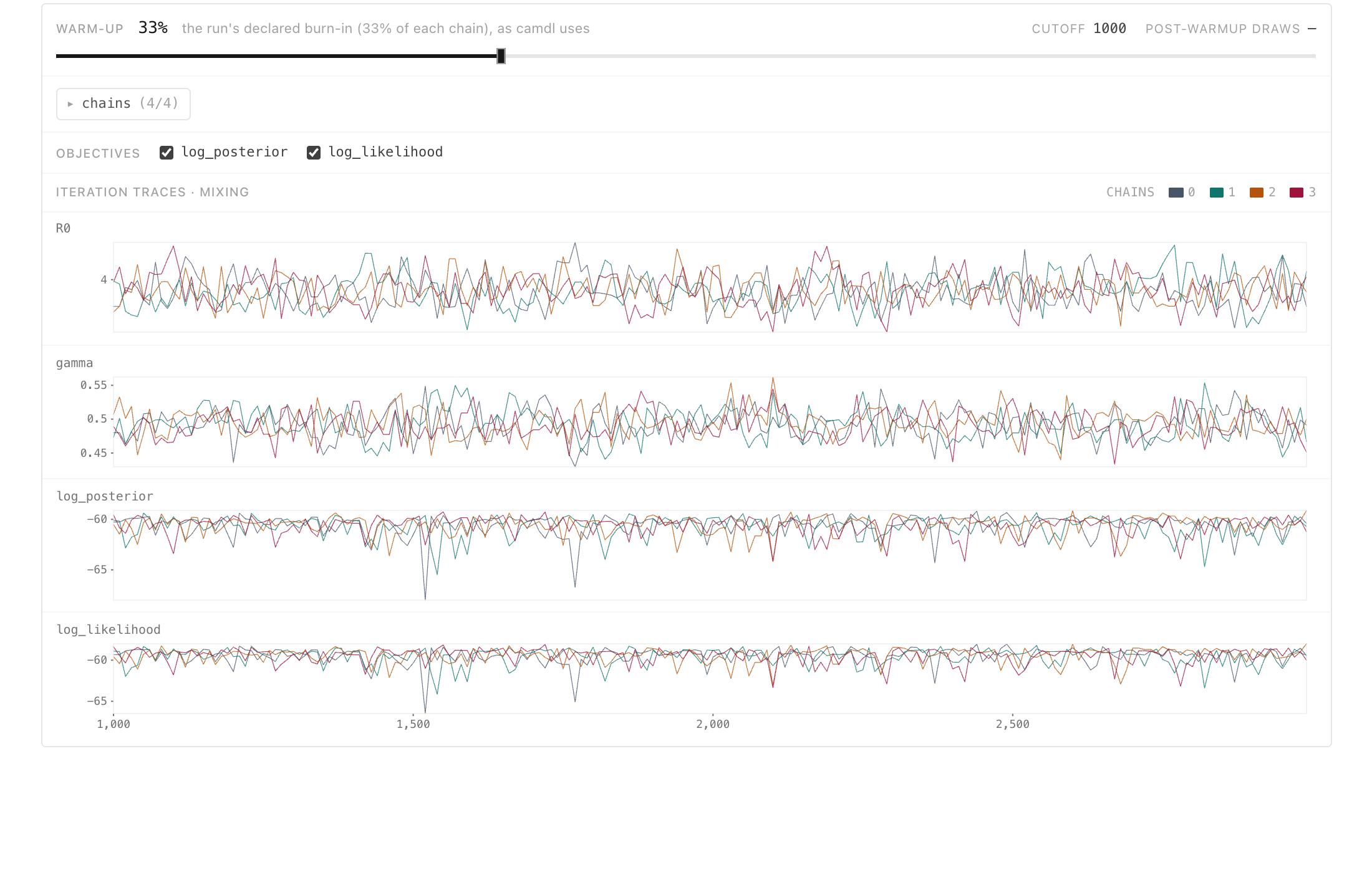
r0 fit in camdl ’scope: the value of each parameter, and the log posterior and log-likelihood, at every step after burn-in, one color per chain.
The four chains move over the same band, and none of them drifts or sits flat for long. That is what the acceptance rates and \hat R summarize. The Pair tab shows the posterior itself:
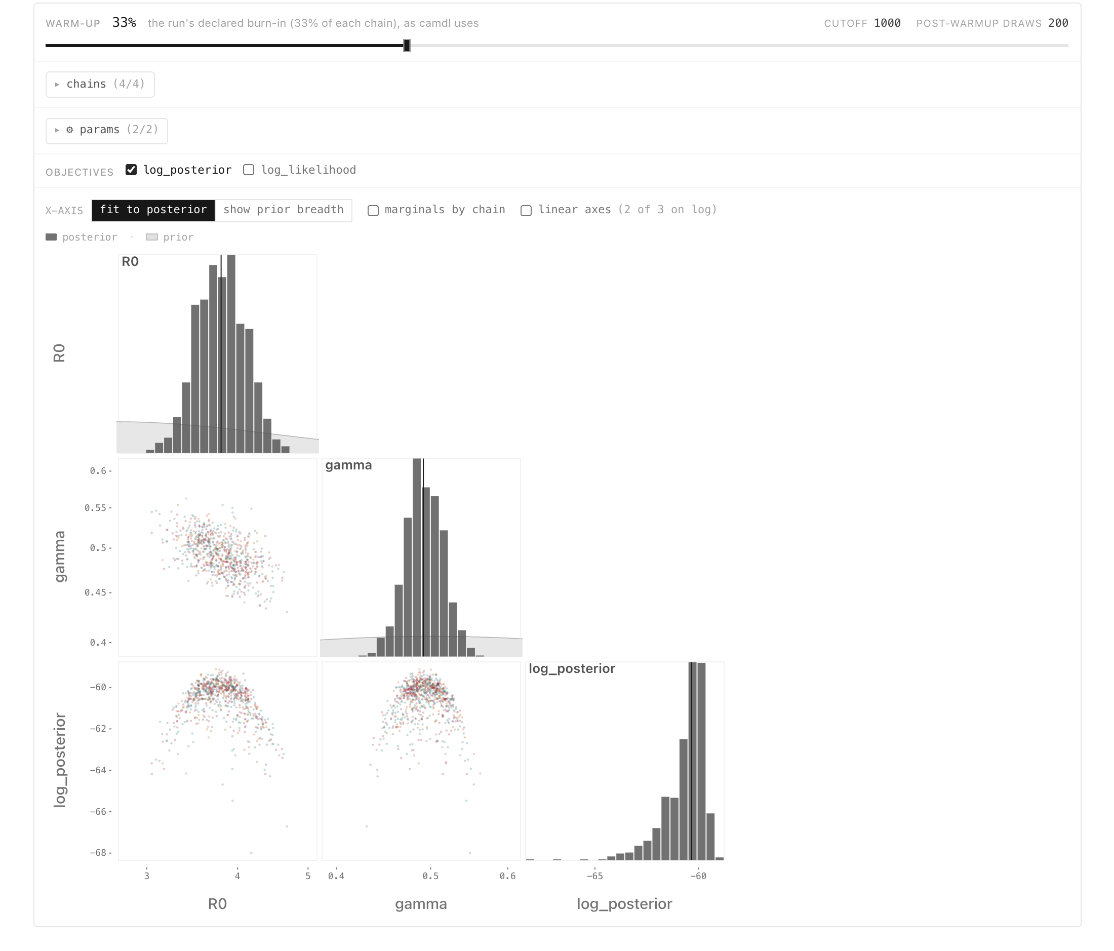
r0 fit: the marginal posterior of each parameter on the diagonal, with the prior shaded behind it, and the draws of each pair of quantities below.
Each marginal posterior is a narrow peak over a prior that, on this scale, is nearly flat: fourteen counts pin both parameters far more tightly than the priors did. R_0 and \gamma are negatively correlated. The epidemic’s early growth rate is roughly \gamma(R_0-1), so a slightly faster recovery paired with a slightly lower R_0 produces almost the same rise; the data constrain the combination better than either parameter alone.
The Diagnostics tab gathers the sampler’s own measurements: camdl’s verdict (read from the run, not recomputed), acceptance per chain against the healthy band, the longest run of consecutive rejected proposals in each chain, and the effective sample size of each parameter by chain. The longest run of rejections is the one to watch in a PMMH fit. A chain whose likelihood estimate once came out far too high rejects everything after it, and an average acceptance rate can hide such a stall. Here the longest is 14 steps.

r0 fit.
The tab’s per-chain acceptance rates are computed over the 200 draws each chain kept, not over all 2000 post-burn-in steps, so they differ from the rates in camdl fit run’s table. Its effective sample sizes per parameter are the summary’s.
Does the fitted model reproduce the data?
Convergence says the sampler found the posterior. Whether the model describes the school is a separate question. A posterior predictive check asks it directly: simulate the epidemic from posterior draws, add the observation noise, and see whether the observed counts look like a typical simulation. fit predict does this two ways. The free_forward horizon simulates each epidemic from day 0 without looking at the data. The one_step horizon predicts each day’s count from the particle filter’s picture of the epidemic given the counts up to the day before.
camdl fit predict @r0
uv run plot_predictive.py ppc-r0.svg Poisson=results/fits/fit_r0-*/predict/*/
fit predict: free_forward horizon — subsampling 200 of 800 posterior draws (raise with --n-draws)
fit predict: one_step horizon — subsampling 200 of 800 posterior draws (raise with --n-draws)
...
wrote results/fits/fit_r0-b7a62cb1/predict/1df66e309ce8/predictive/in_bed.tsv
...fit predict writes its quantiles under the fit’s directory, in predictive/, next to the observed counts in observed/; plot_predictive.py draws them.
The free-forward band (left) is wide, because an epidemic that happens to take off a day early or late stays early or late. The observed epidemic, its rise, its peak of 298 boys on day 5 and its decline, falls inside the 90% band on 13 of the 14 days. The one-day-ahead band (right) is narrow, because it knows where the epidemic was the day before, and only 10 of the 14 counts fall inside it; the misses are all in the decline. Given the epidemic up to yesterday, the model is too sure of today’s count, and the school’s epidemic ended more abruptly than the model’s.
So the fit is sound and the model is close, but not right. Two things are suspect: the Poisson distribution, which allows too little day-to-day scatter, and the SIR dynamics, which end the epidemic too slowly.
Where to go next
The fit on this page went smoothly because of a choice made before it started: the prior on R_0. When a fit goes wrong puts the prior on \beta instead, watches the same sampler fail, works out why, and checks that the fitting machinery recovers parameters it knows. Checking and comparing models takes up the misses in the decline: it fits a model with noisier counts, compares the two, and finds a quantity on which both disagree with the historical record.
The fit workflow lists the steps a larger fit adds, and The reasoning behind the fit workflow explains why each check is there.